The typical flight operation of an airplane involves several phases, and inevitably will include the takeoff, climb, cruise, turns or maneuvers, descent, and finally a landing. As shown in the figure below, a commercial airliner spends much of the duration of its flight in the cruise condition flying from one point to another, which is a predominantly level flight condition at a relatively constant airspeed and relatively high altitude.

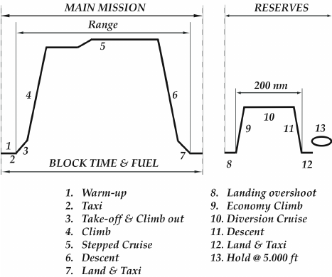
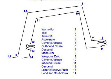
However, a military airplane may spend much more time in climbs, turns, and maneuvers, and the cruise segment may be much shorter and involve an out-and-return mission profile, i.e., fly to a destination to conduct some operation and return to base without landing. Nevertheless, the steady level flight performance of any type of airplane is important in determining its flight range at normal cruising speeds, ceilings, and the airspeeds to fly to attain maximum range and/or endurance.

The analysis pursued to quantify level flight performance depends on the type of airplane, i.e., jet-propelled airplanes or propeller-driven airplanes. For this reason, powerplants have previously classified engines into two main groups; one is propeller-driven engines (i.e., piston-prop and turboprop), and the another one is jet engines (i.e., turbojet and turbofan). The main difference to consider in the analysis of airplane flight performance is that the output of a jet engine is quantified in terms of its thrust production, while the output of an engine driving a propeller is quantified in terms of its power output. However, it must also be recognized that for propeller-driven engines, the power is converted into propulsive thrust by the propeller, and for jet engines, power is required to produce the thrust by increasing the momentum of the flow through the engine in the form of a jet velocity. Therefore, all engines are examined one way or another as power-producing devices, which is why they are all called powerplants. Also, recognize that fuel is required to produce the power, so for airplane performance, the fuel flow and hence the fuel burn is always at the heart of the analysis.

Performance Curves for an Airplane

The performance characteristics of an airplane depend on its aerodynamic drag as well as the characteristics of the engines that power it. A large fraction of the total aircraft drag comes from the wing, which depends primarily on its angle of attack and operational Mach number. However, the airframe drag (everything other than the wing), is also a significant contributor to the total drag of the airplane. Once the drag (or an estimate for drag) is determined, then the thrust or power requirements for flight can be determined at any given weight and altitude (specifically the density altitude). Using the engine characteristics (thrust developed or power available), then many performance characteristics of the airplane can be calculated such as its fuel burn, maximum and minimum attainable flight speeds, rates of climb, best range airspeeds, etc.

The simplest drag model for an airplane is to represent its drag as an average value combined with a value that varies with the square of the lift coefficient. The average value is independent of lift and, in aggregate, accounts for the profile drag on all airframe surfaces, i.e., the sum of the skin friction and pressure drag over the wings, fuselage, empennage, etc. The other part of the total drag is called induced drag because it is the drag that is induced on the airplane from the creation of lift; the physics behind this component is tied to the trailing vortex system behind the airplane, as previously discussed. There are other sources of drag, such as wave drag (from the creation of shock waves). The growth of wave drag as the transonic flight regime is approached is highly nonlinear in terms of Mach number and angle of attack, so the development of a suitable mathematical model is more difficult.

Therefore, for now without wave drag being considered, the drag coefficient for the entire airplane can be expressed as
\begin{equation}
C_D = C_{D_{0}} + C_{D_{i}} = C_{D_{0}} + k C_L^2
\end{equation}
where $C_{D_{i}} $ is the induced drag coefficient and $k$ depends on the wing design. Theoretically, the induced drag coefficient can be expressed as
\begin{equation}
C_{D_{i}} = \frac{C_L^2}{\pi A\!R e} = k C_L^2
\end{equation}
where $A\!R$ is the aspect ratio of the wing and $e$ (the value of $e$ is always < 1) is called Oswald’s wing efficiency factor. The total (dimensional) drag on the airplane is then
\begin{equation}
D = \frac{1}{2} \rho V_{\infty}^2 S \left( C_{D_{0}} + k C_L^2 \right)
\end{equation}
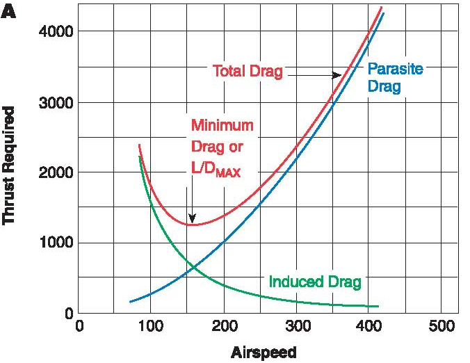
the variation being shown in the figure below, which must be equal to the thrust needed from the propulsive system when lift equals weight, i.e., in trim then
\begin{equation}
L = W, \quad \quad T = D
\end{equation}

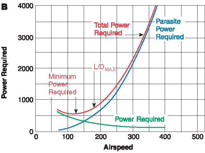
The corresponding power required for flight is then
\begin{equation}
P_{\rm req} = T V_{\infty}
\end{equation}
as shown in the figure below.

Jet-Propelled Airplane

Consider first a jet-propelled airplane. For the steady condition that $T = D$, then
\begin{equation}
T = \frac{1}{2} \rho V_{\infty}^2 S C_D = \frac{1}{2} \rho V_{\infty}^2 S \left( C_{D_{0}} + k C_L^2 \right)
\label{thrust1}
\end{equation}
which assumes that there is no compressibility drag (wave drag) at high cruise Mach numbers. The equation to be solved is
\begin{equation}
T – \frac{1}{2} \rho V_{\infty}^2 S \left( C_{D_{0}} + k C_L^2 \right) = 0
\label{thrust2}
\end{equation}
Because in steady flight $L = W$ then
\begin{equation}
L = \frac{1}{2} \rho V_{\infty}^2 S C_L = W
\end{equation}
where $\rho$ is the density of the air in which the aircraft is flying, $S$ is the reference wing area and $C_L$ is the total wing lift coefficient (the assumption here being that all lift is generated by the wings). Notice that $\rho = \rho_0 \sigma$ where $\sigma$ comes from the ISA model, i.e.,
\begin{equation}
L = W = \frac{1}{2} \rho_0 \sigma V_{\infty}^2 S C_L
\end{equation}
Rearranging this equation the lift coefficient that needs to be produced on the wing for a given flight speed can be solved for, i.e.,
\begin{equation}
C_L = \frac{2 W}{\rho_0 \sigma S V_{\infty}^2}
\label{CLeqn4}
\end{equation}
Therefore, after some algebra the drag becomes
\begin{equation}
D = \frac{1}{2} \rho_0 \sigma V_{\infty}^2 S C_{D_{0}} + \frac{2 k W^2}{\rho_0 \sigma S V_{\infty}^2}
\end{equation}

Notice that the first term in this latter equation (the profile or zero-lift drag) becomes dominant at higher airspeeds, and the second term (the induced drag) becomes larger at lower airspeeds; the resulting drag curve is U-shaped. Therefore, the equation to be solved is
\begin{equation}
T – \frac{1}{2} \rho_0 \sigma V_{\infty}^2 S C_{D_{0}} + \frac{2 k W^2}{\rho_0 \sigma S V_{\infty}^2} = 0
\label{thrust3}
\end{equation}
Of course, this problem can be solved graphically.

Now consider the engine thrust. The thrust from a jet engine decreases proportionally to the air density; for an increase in altitude, the density decreases and the thrust available decreases for a given throttle setting. Throttle settings are generally specified as: takeoff, maximum continuous, cruise, and idle, but military aircraft may have an afterburner selection too.

Clearly, the thrust available (the output of the jet engine) depends on many things, but specifically the airspeed, the density of the air in which the airplane is flying (i.e., the density altitude), and the throttle setting ($\delta_{T_A}$). Therefore, the available thrust from the engine can be written the general form
\begin{equation}
T_A = f(V_{\infty}, \sigma, \delta_{T_A}) \quad \text{or} \quad T_A = f(M_{\infty}, \sigma, \delta_T)
\end{equation}

Consequently, for a given density altitude, airplane weight, and engine throttle setting, both the thrust available (from the engine) and the thrust required (equal to the aircraft drag) becomes a function of airspeed or Mach number. To achieve level flight, then the horizontal equilibrium equation must be satisfied (Eq. \ref{thrust2} or Eq. \ref{thrust3}) for a given weight and altitude. To solve the equation, both the thrust available from the engine and also the thrust required (i.e., the drag of the aircraft) must be plotted versus the airspeed (or Mach number) and then determine the precise conditions where the curves coincide, as shown in the figure below. At that point, Eq. \ref{thrust3} will be satisfied, and both the airspeed and the thrust required for that condition can be determined. Notice in this case that there is a more rapid increase in the thrust required above 500 kts, which is because of the onset of transonic flow and the occurrence of wave drag.

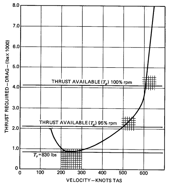
Notice that, potentially, the matching thrust available and thrust required curve can intersect at two points. The intersection at the highest airspeed will correspond to the maximum level flight airspeed for that aircraft at that particular density altitude, aircraft weight, and throttle setting and flight. The intersection at the lower airspeed will be the minimum possible airspeed the aircraft can maintain level flight at that altitude and is called the thrust-limited minimum airspeed, which in some cases may be higher than the stall airspeed. In general, the actual minimum flyable airspeed of an airplane at a given altitude will be the greater of either the thrust-limited minimum airspeed or the stall speed, but in the clean configuration (no flaps), the stall speed is usually the higher speed.

Proceeding further, the thrust available, and thrust required curves versus airspeed can be plotted for each altitude of interest. Of course, the exact quantitative relationships between power and airspeed depend on the detailed aerodynamics of the actual airplane as well as the characteristics of the engines, which as previously mentioned may not be available other than in numerical form, e.g., tables. As altitude increases and the air density decreases, the thrust available at a given throttle setting decreases, as shown in the figure below then these points represent the maximum and minimum airspeeds that the aircraft can fly at each altitude for the given weight and throttle setting and so determine the maximum speed flight envelope. Notice that at higher altitudes, the achievable lowest airspeed becomes thrust limited, while at the lower altitudes, the achievable speed is determined by stall.

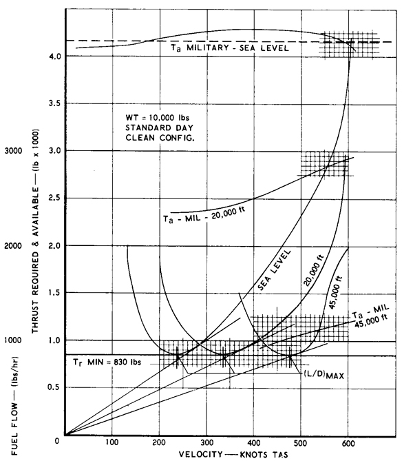
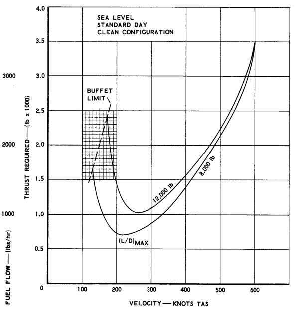
It can also be seen that there will eventually be some altitude at which the available thrust approaches the minimum drag where the available thrust curve will just touch the thrust required curve at a single point. This condition corresponds (more or less) to the achievable maximum altitude or ceiling of the aircraft. Changing the weight of the aircraft has a large effect on the thrust curves because the lift coefficient increases, and so the induced drag increases at lower airspeeds. As shown in the figure below, increasing flight weight tends to shift the thrust required curve up and to the right.

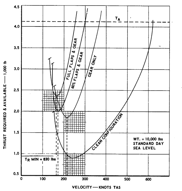
The effect of configuration also has an effect on the thrust required, as shown in the figure below. The clean configuration is the normal flight condition with flaps and landing gear retracted. Lowering the landing gear gives a large increase in drag, and the deployment of the flaps increases this drag further. Notice that the flight envelope (or corridor) is increasingly constrained between the thrust available from the engines and the stall speed of the aircraft. Such narrow airspeed bands require that the aircraft be flown fairly precisely during landing.

While these forgoing graphical results are fairly easy to see, the problem can also be solved analytically under some conditions. Take as a further example a jet-powered airplane where it can be assumed that the propulsive thrust is not strongly dependent on the airspeed for a given altitude, i.e., where it is reasonable to assume that $T = $ constant for a given altitude. The speed of the airplane can be found from
\begin{equation}
T – \frac{1}{2} \rho S \left( C_{D_{0}} + k C_L^2 \right) V_{\infty}^2 = 0
\end{equation}
After some algebra and rearrangement of terms, the airspeed for thrust and drag equilibrium can be obtained by solving the quartic equation
\begin{equation}
c_1 V_{\infty}^4 + c_2 V_{\infty}^2 + c_3 = 0
\label{quartic}
\end{equation}
where
\begin{equation}
c_1 = -\frac{1}{2} \rho_0 \sigma \frac{S}{W} C_{D_{0}}, \quad c_2 = \frac{T}{W}, \quad c_3 = -k \frac{2}{\rho_0 \sigma} \frac{W}{S}
\end{equation}
Notice that these coefficients contain both the thrust to weight ratio and the wing loading. While there are multiple roots to Eq. \ref{quartic} they are not all physical, and only two roots will have physical significance. It can be shown that the jet airplane can maintain level flight at a given altitude if
\begin{equation}
\frac{T}{W} \ge 2 \sqrt{C_{D_{0}} k}
\end{equation}
which is naturally and intrinsically tied to the aerodynamic characteristics of the aircraft. The limiting condition of this latter result occurs at the ceiling of the aircraft when the minimum and maximum attainable airspeeds coincide, which is
\begin{equation}
V_{\infty} = -\frac{c_2}{2 c_1} = \frac{T}{\rho_0 \sigma S C_{D_{0}}}
\end{equation}
However, this value can only be determined explicitly if the engine thrust is known, which, as previously discussed, is a function of density altitude and throttle setting.

In most cases, the foregoing type of problem must be solved numerically or graphically. The procedures described would apply to any drag or thrust variations. The propulsion characteristics of engines are often made available for engineering analysis in terms of graphs and/or tables to allow the thrust at each airspeed and altitude to be calculated. Similar procedures are used to develop a more detailed model of the drag on the aircraft, including the effects of wave drag. For high-performance aircraft, such results are usually determined using a combination of calculations, wind tunnel tests, and flight tests and are made available as tables as functions of the angle of attack and Mach number.

Propeller Driven Airplane

Consider now a propeller-driven airplane. Remember that the output of an engine driving a propeller (e.g., a turboshaft) is quantified in terms of its power, although it must also be recognized that this power is converted into thrust through the aerodynamic performance of the propeller. There may be some jet thrust from a turboshaft, but usually, this is small enough to be ignored.

The power required for flight can be written as
\begin{equation}
P_{\rm req} = \frac{T V_{\infty}}{\eta_p} = \frac{1}{\eta_p} \left( \frac{1}{2} \rho V_{\infty}^3 S \left( C_{D_{0}} + k C_L^2 \right) \right)
\label{power1}
\end{equation}
where $\eta_p$ can be considered as the net propulsive efficiency of the propulsive system (engine and propeller combined); notice that this value may not be a constant and will generally vary with airspeed depending on the type of propeller system. Splitting the foregoing equation (Eq. \ref{power1}) into its two parts leads to
\begin{equation}
P_{\rm req} = \frac{1}{\eta_p} \left( \frac{1}{2} \rho V_{\infty}^3 S C_{D_{0}} \right) + \frac{k}{\eta_p} \left( \frac{1}{2} \rho V_{\infty}^3 S C_L^2 \right)
\end{equation}
the first part being the non-lifting part and the second being the induced part. Notice that the power associated with the non-lifting part increases with the cube of the airspeed but the second (induced) part depends on the lift coefficient, which as has previously been shown, reduces with the airspeed.

Using Eq. \ref{CLeqn4} gives
\begin{equation}
C_L^2 = \left(\frac{2 W}{\rho_0 \sigma S V_{\infty}^2}\right)^2
\end{equation}
so the power required equation now becomes
\begin{equation}
P_{\rm req} = \left(\frac{1}{2} \rho_0 \sigma V_{\infty}^3 S \right) \frac{1}{\eta_p} C_{D_{0}} + \frac{1}{2} \rho_0 \sigma V_{\infty}^3 S \left( \frac{k}{\eta_p} \right) \left(\frac{2 W}{\rho_0 \sigma S V_{\infty}^2}\right)^2
\end{equation}
which after some simplification leads to
\begin{equation}
P_{\rm req} = \left( \frac{1}{2} \rho_0 \sigma V_{\infty}^3 S \right) \frac{1}{\eta_p} C_{D_{0}} + \left( \frac{k}{\eta_p} \right) \frac{2 W^2}{\rho_0 \sigma S V_{\infty} }
\label{powereqn}
\end{equation}
which is simply in the form
\begin{equation}
P_{\rm req} = A V_{\infty}^3 + \frac{B}{V_{\infty}}
\label{powereqn2}
\end{equation}
where
\begin{equation}
A = \frac{1}{2} \rho_0 \sigma \frac{1}{\eta_p} C_{D_{0}}
\label{A}
\end{equation}
and
\begin{equation}
B = \frac{k}{\eta_p} \frac{2 W^2}{\rho_0 \sigma S}
\label{B}
\end{equation}
Notice that the non-lifting part increases with the cube of the airspeed but the lifting part decreases inversely with airspeed.

A representative power curve is shown in the figure below, with higher power being required at lower airspeeds, some minimum range of power at some intermediate airspeeds, and then a rapid increase in power (with the cube of the airspeed) as higher airspeeds are reached. Aircraft that use propellers usually depend on performance charts that are given in terms of airspeed rather than Mach number. Like the jet-powered airplane, the lowest possible airspeed is limited by the onset of wing stall, no matter how much power (or thrust) is available. At higher weights and/or density altitudes, it is the rapid increase in power required that will eventually limit the maximum level flight airspeed of the airplane for a given weight and operational altitude, that is, assuming no other barrier to flight appears.

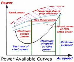
The power available typically increases rapidly with airspeed and levels off over the airspeed range where the airplane would normally fly. Again, analogous to the manner for the jet aircraft, the level flight solution is the intersection of the power available curves and power required curves. The highest airspeed solution is the maximum level flight airspeed (at a given altitude, aircraft weight, and throttle setting). However, the minimum speed solution is only valid if that speed is greater than the stall speed of the aircraft. Again, the ceiling of the aircraft can be determined in this case at the airspeed when the minimum power for flight coincides with the power available.

By assuming that $k$ and the propulsive efficiency $\eta_p$ remain constant for all weights and airspeeds then the airspeeds can be solved for in closed form. This is a special case, admittedly, but a reasonable assumption for a constant speed propeller with the engine operating at wide-open throttle. After some algebra, the needed equation to be solved is
\begin{equation}
c_1 V_{\infty}^3 + \frac{c_2}{V_{\infty}} + c_3 = 0
\end{equation}
where
\begin{equation}
c_1 = -\frac{1}{2} \frac{\rho_0 \sigma S C_{D_{0}}}{W}, \quad c_2 = -2 k \left( \frac{W}{\rho_0 \sigma S} \right), \quad c_3 = \frac{\eta_p P_{\rm req}}{W}
\end{equation}
from which the maximum and minimum speeds can, in principle, be solved for. However, recognize that this is a more difficult problem to solve because the relevant equation is nonlinear.